Introduction to PostgreSQL Indexes ::

Who’s this for

This text is for developers that have an intuitive knowledge of what database indexes are, but don’t necessarily know how they work internaly, what are the tradeoffs associated with indexes, what are the types of indexes provided by postgres and how you can use some of its more advanced options to make them more optimized for your use case.

Basics

Indexes are special database objects primarily designed to increase the speed of data access, by allowing the database to read less data from the disk. They can also be used to enforce constraints like primary keys, unique keys and exclusion. Indexes are important for performance but do not speedup a query unless the query matches the columns and data types in the index. Also, as a very rough rule of thumb, an index will only help if less than 15-20% of the table will be returned in the query, otherwise the query planner, a part of postgres used to determine how the query is going to be executed, might prefer a sequential scan. In fact, reality is much more complex than this rule of thumb. The query planner uses statistics and predefined costs associated with each type of scan to do its job, but we’re only going approach the query planner behavior tangentially in this article. So, if your query returns a large percentage of the table, consider refactoring it, using summary tables or other techniques before throwing an index at the problem. With that in mind, let’s give a closer look at how Postgres stores your data in the disk and how indexes help to speedup querying this data.

There are six types of indexes available in the default postgres installation and more types available through extensions. Typically, they work by associating a key value with a data location in one or more rows of the table containing that key. Each line is identified by a TID, or tuple id.

How data is stored in disk

To understand indexes, it is important to first understand how postgres stores table data on disk. Every table in postgres has one or more corresponding files on disk, depending on its size. This set of files is called a heap and it is divided into 8kb pagesh. All table rows, internally referred to as “tuples”, are saved in these files and do not have a specific order. The index is a tree structure that links the indexes columns to the row locators, also known as ctid, in the heap. We’ll zoom into the index internals later.

To see the heap files we can use a few postgres internal tables to see where they’re located in the disk. First, we can enter psql and use show data_directory to show the directory Postgres uses to store databases physical files.

 show data_directory;

         data_directory          
---------------------------------
 /opt/homebrew/var/postgresql@16

Now we can use the internal pg_class to find the file where the heap table is stored:

create table foo (id int, name text);


select oid, datname
from pg_database
where datname = 'my_database';                                                                                

  oid  |         datname        
-------+-------------------------
 71122 | my_database
(1 row)

select relfilenode from pg_class where relname = 'foo';                                                                                                  
 relfilenode
-------------
       71123

Finally, we can check the file on disk by running this command in the shell (ls $PGDATA/base/<database_oid>/<table_oid>):

ls -lrt /opt/homebrew/var/postgresql@16/base/71122/71123
-rw-------  1 dlt  admin  0 16 Aug 14:20 /opt/homebrew/var/postgresql@16/base/71122/71123

The file has size 0 because we haven’t done any INSERTs in this table yet.

Let’s add a couple of rows to our table:

insert into foo (id, name) values (1, 'Ronaldo');
INSERT 0 1
insert into foo (id, name) values (2, 'Romario');
INSERT 0 1

We can add the ctid field to the query to retrieve the ctid of each line. The ctid is an internal field that has the address of the line in the heap. Think of it as a pointer to the row location in the heap. It consists of a tuple in the format (m, n) where m is the block id and n is the tuple offset. “ctid” stands for “current tuple id”. Here you can note that the row with id one is stored in the page 0, offset 1.

select ctid, * from foo;
 ctid  | id |  name   
-------+----+---------
 (0,1) |  1 | Ronaldo
 (0,2) |  2 | Romario
(2 rows)

How indexes speedup access to data

Let’s add more players to the table so that the total rows is one million:

insert into foo (id, name);
select generate_series(3, 1000000), 'Player ' || generate_series(3, 1000000);

After adding more rows to the table its corresponding file is 30MB. Internally, it is divided into 8kb pages.

ls -lrtah /opt/homebrew/var/postgresql@16/base/71122/71123
-rw-------  1 dlt  admin    30M 16 Aug 16:32 /opt/homebrew/var/postgresql@16/base/71122/71133

When we query a table without an index, Postgres reads all tuples in every page and apply a filter. For example, let’s analyze the command below that searches for rows whose name column value is equal to “Ronaldo” and show how the database performed this search. We use the explain command with the options (analyse, buffers). analyse will actually execute the query instead of just using cost estimates, and the buffers option shows how much IO work was done.

 explain (analyze, buffers) select * from foo where name = 'Ronaldo';
                                                     QUERY PLAN
---------------------------------------------------------------------------------------------------------------------
 Gather  (cost=1000.00..12577.43 rows=1 width=18) (actual time=0.307..264.991 rows=1 loops=1)
   Workers Planned: 2
   Workers Launched: 2
   Buffers: shared hit=97 read=6272
   ->  Parallel Seq Scan on foo  (cost=0.00..11577.33 rows=1 width=18) (actual time=169.520..256.639 rows=0 loops=3)
         Filter: (name = 'Ronaldo'::text)
         Rows Removed by Filter: 333333
         Buffers: shared hit=97 read=6272
 Planning Time: 0.143 ms
 Execution Time: 265.021 ms

Note the in output the line starting with " -> Parallel Seq scan on foo". This line denotes that the database performed a sequential search and read all the rows in the table. The execution time for this query was 265.021ms. Also note the line that says “Buffers: shared hit=97 read=6272”. This mean that we needed to read 97 pages from memory, and 6272 pages from disk.

Now let’s add an index on the name column and see how the same query performs. We’re using the command create index concurrently because we don’t want to block the table for writes.

create index concurrently on foo(name);
CREATE INDEX

explain (analyze, buffers) select * from foo where name = 'Ronaldo';
                                                    QUERY PLAN
-------------------------------------------------------------------------------------------------------------------
 Index Scan using foo_name_idx on foo  (cost=0.42..8.44 rows=1 width=18) (actual time=0.047..0.049 rows=1 loops=1)
   Index Cond: (name = 'Ronaldo'::text)
   Buffers: shared hit=4
 Planning Time: 0.129 ms
 Execution Time: 0.077 ms
(5 rows)

Here we see that the index was used and that in this case the execution time was reduced from 264.21 to 0.074 milliseconds, and the database only needed to read 4 pages! The reduction in execution time happens because, now, instead of reading all the rows in the table, the database uses the index. The index is a tree structure mapping the value “Ronaldo” to the ctid(s) of the rows that have this value in the name column (in our example we only have one such row). The ctid is then used to quickly locate these rows on the heap.

If we use \di+ to show the indexes in our database we can see that the index we’ve created occupies 30MB, roughly the same size as the foo table.

\di+

                                         List of relations
 Schema |     Name     | Type  | Owner | Table | Persistence | Access method | Size  | Description
--------+--------------+-------+-------+-------+-------------+---------------+-------+-------------
 public | foo_name_idx | index | dlt   | foo   | permanent   | btree         | 30 MB |
(1 row)

Costs associated with indexes

It is important to highlight that the extra speed brought by indices is associated with several costs that must be considered when deciding where and how to apply them.

Disk Space

Indexes are stored in a separate area of the heap and take up additional disk space. The more indexes a table has, the greater the amount of disk space required to store them. This incurs in additional storage costs for your database and for backups, increased replication traffic, and increased backup and failover recovery times. Bear in mind that its not uncommon for btree indexes to be larger than the table itself. Learning about partial indexes, and multicolumn indexes, as well as about other more space efficient index types such as BRIN can be helpful.

Write operations

Also, there is a maintenance cost in writing operations such as UPDATE, INSERT and DELETE, if a field that is part of an index is modified, the corresponding index needs to be updated, which can add significant overhead to the writing process.

Query planner

The query planner (also known as query optimizer) is the component responsible for determining the best execution strategy for a query. With more indexes available, the query planner has more options to consider, which can increase the time needed to plan the query, especially in systems with many complex queries or where there are many indexes available.

Memory usage

PostgreSQL maintains a portion of frequently accessed data and index pages in memory in its shared buffers. When an index is used, the relevant index pages are loaded into shared buffers to speed up access. The more indexes you have and the more they are used, the more shared buffer memory is necessary. Since shared buffers are limited and are also used for caching data pages, filling the shared buffers with indexes can lead to less efficient caching of table data. It’s also good to keep in mind that the whole indexed column is copied in every node of the btree, since there’s a limit in node size capacity, the larger the indexed column the deeper the tree will be.

Another aspect of memory usage is that PostgreSQL uses work memory when it executes queries that involves sorting or complex index scans (involving multi-column or covering indexes). Larger indexes require more memory for these operations. Also, indexes require memory to store some metadata about their structure, column names and statistics in the system catalog cache. And finally indexes require memory for maintainance operations like vacuuming and reindexing operations.

Types of Indexes

Btree

The B-Tree is a very powerful data structure, present not only in Postgres but in almost every database management system, since it is a very good general purpose index. It was invented by Rudolf Bayer and Edward M.McCreight while working at Boeing. Nobody really knows if the “B” in B-tree stands for Bayer, Boeing, balanced or better, and it doesn’t really matter. What really matters is that it enables us to search elements in the tree in O(log n) time. If you’re not familiar with Big-O notation, all you need to know is that is is really fast - you only need to make 20 comparisons in order to find an element in a set with 1 million items. Moreover, it can maintain O(log n) time complexity for data sets that are larger than the RAM available on a computer. This means that disks can be used to extend RAM, thanks to the btree efficient prevention of disk page accesses to find the desired data. In PostgreSQL the btree is the most common type of index and its the default, it’s also used to support system and TOAST indexes. Even an empty database has hundreds of btree indexes. It is the only index type that can be used for primary and unique key constraints.

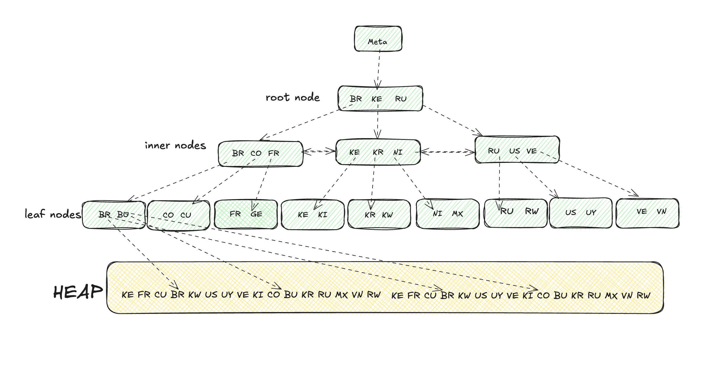
In contrast with a binary tree, the BTree is a balanced tree and all of its leave nodes have the same distance from the root. The root nodes and inner nodes have pointers to lower levels, and the leaf nodes have the keys and pointers to the heap. Postgres btrees also have pointers to the left and right nodes for easier forward and backward scanning. Nodes can have multiple keys and these keys are sorted so that it’s easy to walk in ordered directions and to perform ORDER BY and JOIN operations. The values are only stored in the leaf nodes, this makes the tree more compact and facilitates a full traversal of the objects in a tree with just a linear pass through all the leaf nodes. This is just a simplified description of PostgreSQL Btree indexes, if you want to get into the low level details, I suggest you to read the README and the paper that inspired them. Below there’s a simplified illustration of a Postgres Btree.

postgres btree

Using multiple indexes

Postgres can use multiple indexes to handle cases that cannot be handled by single index scans, by forming AND and OR conditions across several index scans with the support of bitmaps. The bitmaps are ANDed or ORed together as needed by the query and finally the table rows are visited and returned. Let’s say we have a query like this:

select * from users where age = 30 and login_count = 100;

If the age and login_count columns are indexed, postgres scans index age for all pages with age=30 and makes a bitmap where the pages that might contain rows with age=30 are true. In a similar way, it builds a bitmap using the login_count index. It then ANDs the two bitmaps to form a third bitmap, and performs a table scan, only reading the pages that might contain candidate values, and only adding the rows where age=30 and login_count=100 to the result set.

Multi-column indexes

Multi-column indexes are an alternative for using multiple indexes. They’re generaly going to be smaller and faster than using multiple indexes, but they’ll also be less flexible. That’s because the order of the columns matter, because the database can search for a subset of the indexed columns, as long as they are the leftmost columns. For example, if you have an index on column a and another index on column b, these indexes will serve all the of queries below:

select * from my_table where a = 42 and b = 420;

select * from my_table where a = 43;

select * from my_table where b = 99;

On the other hand, only the first two queries would use an index if you created a multi-column index on (a, b) with a command like create index on my_table(a, b); So, when building multi-column indexes choose the order of the columns well so that your index can be used by the most queries possible.

Partial indexes

Partial indexes allow you to use a conditional expression to control what subset of rows will be indexed, this can bring you many benefits:

your index can be smaller and more likely fit in RAM.
your index is shallower, so lookups are quicker
less overhead for index/update/delete (but can also mean more overhead if the column you’re using to filter rows in/out of the index is updated very frequently triggering constant index maintenance)

They’re mostly useful in situations where you don’t care about some rows, or when you’re indexing on a column where the proportion of one value is much greater than others. I’ll give two examples below.

When you don’t care about some rows

Let’s say you have a rules table where the rows can be marked as enabled/disabled, the vast majority of the rows are disabled and in your queries you only care about enabled rows. In this case, you would have a partial index, filtering out the disable rows like this:

create index on rules(status) where status = 'enabled';

When the distribution of values is skewed

Now imagine you’re building a todo application and the status column value can be either TODO, DOING, and DONE. Suppose you have 1M rows and this is the current distribution of rows in each status:

Rows	Status
TODO	90%
DOING	5%
DONE	5%

Since postgres keeps statistics about the distribution of values in your table columns and knows that the vast majority of the rows are in the TODO status, it would choose to do a sequential scan on the tasks table when you have status='TODO' in the WHERE clause of your query, even if you have an index on status, leaving most part of the index unused and wasting space. In this case, a partial scan such as the one below is recommended:

create index on tasks(status) where status <> 'TODO';

Covering indexes

If you have a query that selects only columns in an index, Postgres has all information needed by the query in the index and doesn’t need to fetch pages from the heap to return the result. This optimization is called index-only scan. To understand how it works, consider the following scenario:

create table bar (a int, b int, c int);
create index abc_idx on bar(a, b);

/* query 1 */
select a, b from bar;

/* query 2 */
select a, b, c from bar;

In the first query, postgres can do an index-only scan and avoid fetching data from the heap because the values a and b are present in the index. In the second query, since c isn’t in the index, posgres needs to follow the reference to the heap to fetch its value. In the first query we allowed postgres do to an index-only scan with the help of a multi-column index, but we could also achieve the same result by using a covering index. The syntax for creating a covering index looks like this:

create index abc_cov_idx on bar(a, b) including c;

This is more space efficient than creating a multi-column index on (a, b, c), because c will only be inserted at the leaf nodes of the btree. Also, we might want to use a covering index in cases where we want an unique index and c would “break” the uniqueness of the index.

Expression indexes

Expression indexes to index the result of an expression or function, rather than just the raw column values. This can be extremely useful when you frequently query based on a transformed version of your data. It is necessary if you use a function as part of a where clause as in the example below:

CREATE TABLE customers (
    id SERIAL PRIMARY KEY,
    name TEXT
);

CREATE INDEX idx_name ON customers(name);
SELECT * FROM customers WHERE LOWER(name) = 'john doe';

In this example above, Postgres won’t use the index because it was was built against the name column. In order to make it work, the index key has to call the lower function just like it’s used in the where clase. To fix it, do:

Now, when you run a query like this:

CREATE INDEX idx_lower_name ON customers (lower(name));

Now PostgreSQL can use the expression index to efficiently find the matching rows.

Expression indexes can be created using various types of expressions:

Built-in functions: Like lower(), upper(), etc.
User-defined functions: As long as they are immutable.
String concatenations: Like first_name || ' ' || last_name.

Hash

The hash index differs from B-Tree in strucutre, it is much more alike a hashmap data structure present in most programming languages (e.g. dict in Python, array in php, HashMap in java, etc). Instead of adding the full column value to the index, a 32bit hash code is derived from it and added to the hash. This makes hash indexes much smaller than btrees when indexing longer data such as UUIDs, URLs, etc. Any data type can be indexed with the help of postgres hashing functions. If you type \df hash* and press TAB in psql, you’ll see that there are more then 50 hash related functions. Although it gracefully handles hash conflicts, it works better for even distribution of hash values and is most suited to unique or mostly unique data. Under the correct conditions it will not only be smaller than btree indexes, but also it will be faster for reads when compared with btress. Here’s what the official docs says about it:

“In a B-tree index, searches must descend through the tree until the leaf page is found. In tables with millions of rows, this descent can increase access time to data. The equivalent of a leaf page in a hash index is referred to as a bucket page. In contrast, a hash index allows accessing the bucket pages directly, thereby potentially reducing index access time in larger tables. This reduction in “logical I/O” becomes even more pronounced on indexes/data larger than shared_buffers/RAM.”

As for its limitations, it only supports equality operations and isn’t going to be helpful if you need to order by the indexed field. It also doesn’t support multi-column indexes and checking for uniqueness. For a in-depth analysis of how hash indexes fare in relation to btree, check Evgeniy Demin’s blog post on the subject.

BRIN

BRIN stands for Block Range Index and its name tells a lot about how it is implemented. Nodes in BRIN indexes store the minimum and maximum values of a range of values present in the page referred by the index. This makes the index more compact and cache friendly, but restricts the use cases for it. If you have a very large in a work load that is heavy on writes and low on deletes and updates. You can think of a BRIN index as an optimizer for sequential scans of large amounts of data in very large databases, and is a good optimization to try before partitioning a table. For a BRIN index to work well, the index key should be a column that strongly correlates to the location of the row in the heap.Some good use cases for BRIN are append-only tables and tables storing time series data.

BRIN won’t work well for tables where the rows are updated constantly, due to the nature of MVCC that duplicates rows and stores them in a different part of the heap. This tuple duplication and moving affect the correlation negatively and reduces the effectiveness of the index. Using extensions such as pg_repack or pg_squeeze isn’t recommended for tables that use BRIN indexes, since they change the internal data layour fo the table and mess up the correlation. Also, this index is lossy in the sense that the index leaf nodes point to pages taht might contain a value within a particular range. For this reason a BRIN is more helpful if you need to return large subset of data, and a btree would be more read performant for queries that only return one or few rows. You can make the index more or less lossy by adjusting the page_per_range configuration, the trade off will be index size.

GIN

Generalized inverted index is appropriate for when you want to search for an item in composite data, such as finding a word in a blob of text, an item in an array or an object in a JSON. The GIN is generalized in the sense that it doesn’t need to know how it will acelerate the search for some item. Instead, there’s a set of custom strategies specific for each data type. Please note that in order to index an JSON value it needs to be stored in a JSONB column. Similarly, if you’re indexing text it’s better to store it as (or convert it to) tsvector or use the pg_trgm extension.

GiST & SP-GiST

The Generalized Search Tree and the Space-Partitioned Generalized Search Tree are tree structures that can be use as a base template to implement indexes for specific data types. You can think of them as framework for building indexes. The GiST is a balanced tree and the SP-GiST allow for the development of non-balanced data structures. They are useful for indexing points and geometric types, inet, ranges and text vectors. You can find an extensive list of the built-in strategies shipped with postgres in the official documentation. If you need an index to enable full-text search in your application, you’ll have to choose between GIN and GiST. Roughly speaking, GIN is faster for lookups but it’s bigger and has greater building and maintainance costs. So the right index type for you will depend on your application requirements.

Conclusion

Understanding and effectively using indexes is crucial for optimizing database performance in PostgreSQL. While indexes can greatly speed up query execution and improve overall efficiency, it’s important to be mindful of their impact on write operations and storage. By carefully selecting the appropriate types of indexes based on your specific use cases you can ensure that your PostgreSQL database remains both fast and efficient. I hope this article taught you at least one or two things you didn’t know about Postgres indexes, and that you’re better equiped to deal with different scenarios involving databases from now on.